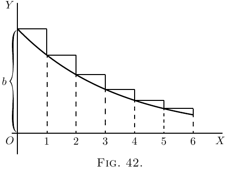
(b)The Die-away Curve
If we were to take $p$ as a proper fraction (less than
unity), the curve would obviously tend to sink downwards,
as in Figure 42, where each successive ordinate
is $\frac{3}{4}$ of the height of the preceding one.
The equation is still
\[
y=bp^x;
\] but since $p$ is less than one, $\log_\epsilon p$ will be a negative
quantity, and may be written $-a$; so that $p=\epsilon^{-a}$,
and now our equation for the curve takes the form
\[
y=b\epsilon^{-ax}.
\]
The importance of this expression is that, in the
case where the independent variable is time, the
equation represents the course of a great many
physical processes in which something is gradually
dying away. Thus, the cooling of a hot body is
represented (in Newton's celebrated “law of cooling”)
by the equation
\[
\theta_t=\theta_0 \epsilon^{-at};
\]
where $\theta_0$ is the original excess of temperature of a
hot body over that of its surroundings, $\theta_t$ the excess
of temperature at the end of time $t$, and $a$ is a constant–namely,
the constant of decrement, depending
on the amount of surface exposed by the body, and
on its coefficients of conductivity and emissivity,
etc.
A similar formula,
\[
Q_t=Q_0 \epsilon^{-at},
\]
is used to express the charge of an electrified body,
originally having a charge $Q_0$, which is leaking away
with a constant of decrement $a$; which constant
depends in this case on the capacity of the body and
on the resistance of the leakage-path.
Oscillations given to a flexible spring die out after
a time; and the dying-out of the amplitude of the
motion may be expressed in a similar way.
In fact $\epsilon^{-at}$ serves as a die-away factor for all
those phenomena in which the rate of decrease
is proportional to the magnitude of that which is
decreasing; or where, in our usual symbols, $\dfrac{dy}{dt}$ is
proportional at every moment to the value that $y$ has
at that moment. For we have only to inspect the
curve, Figure 42 above, to see that, at every part of it,
the slope $\dfrac{dy}{dx}$ is proportional to the height $y$; the
curve becoming flatter as $y$ grows smaller. In symbols,
thus
$y=b\epsilon^{-ax}$ or
\[
\log_\epsilon y
= \log_\epsilon b - ax \log_\epsilon \epsilon
= \log_\epsilon b - ax,\\
\text{and, differentiating,}\;
\frac{1}{y}\, \frac{dy}{dx} = -a;\\
\text{hence}\; \frac{dy}{dx} = b\epsilon^{-ax} × (-a) = -ay;
\]
or, in words, the slope of the curve is downward, and
proportional to $y$ and to the constant $a$.
We should have got the same result if we had
taken the equation in the form
\begin{align*}
y &= bp^x; \\
\text{for then}\;
\frac{dy}{dx}
&= bp^x × \log_\epsilon p. \\
\text{But}\;
\log_\epsilon p &= -a; \\
\text{giving us}\;
\frac{dy}{dx} &= y × (-a) = -ay,
\end{align*}
as before.
The Time-constant. In the expression for the “die-away
factor” $\epsilon^{-at}$, the quantity $a$ is the reciprocal of
another quantity known as “the time-constant,” which
we may denote by the symbol $T$. Then the die-away
factor will be written $\epsilon^{-\frac{t}{T}}$; and it will be seen, by
making $t = T$ that the meaning of $T$ $\left(\text{or of} \dfrac{1}{a}\right)$ is that
this is the length of time which it takes for the original
quantity (called $\theta_0$ or $Q_0$ in the preceding instances)
to die away $\dfrac{1}{\epsilon}$th part–that is to $0.3678$–of its
original value.
The values of $\epsilon^x$ and $\epsilon^{-x}$ are continually required
in different branches of physics, and as they are given
in very few sets of mathematical tables, some of the
values are tabulated here for convenience.
| $x$ |
$\epsilon^x$ |
$\epsilon^{-x}$ |
$1-\epsilon^{-x}$ |
| $0$ | $1.0000$ | $1.0000$ | $0.0000$ |
| $0.10$ | $1.1052$ | $0.9048$ | $0.0952$ |
| $0.20$ | $1.2214$ | $0.8187$ | $0.1813$ |
| $0.50$ | $1.6487$ | $0.6065$ | $0.3935$ |
| $0.75$ | $2.1170$ | $0.4724$ | $0.5276$ |
| $0.90$ | $2.4596$ | $0.4066$ | $0.5934$ |
| $1.00$ | $2.7183$ | $0.3679$ | $0.6321$ |
| $1.10$ | $3.0042$ | $0.3329$ | $0.6671$ |
| $1.20$ | $3.3201$ | $0.3012$ | $0.6988$ |
| $1.25$ | $3.4903$ | $0.2865$ | $0.7135$ |
| $1.50$ | $4.4817$ | $0.2231$ | $0.7769$ |
| $1.75$ | $5.755$ | $0.1738$ | $0.8262$ |
| $2.00$ | $7.389$ | $0.1353$ | $0.8647$ |
| $2.50$ | $12.182$ | $0.0821$ | $0.9179$ |
| $3.00$ | $20.086$ | $0.0498$ | $0.9502$ |
| $3.50$ | $33.115$ | $0.0302$ | $0.9698$ |
| $4.00$ | $54.598$ | $0.0183$ | $0.9817$ |
| $4.50$ | $90.017$ | $0.0111$ | $0.9889$ |
| $5.00$ | $148.41$ | $0.0067$ | $0.9933$ |
| $5.50$ | $244.69$ | $0.0041$ | $0.9959$ |
| $6.00$ | $403.43$ | $0.00248$ | $0.99752$ |
| $7.50$ | $1808.04$ | $0.00055$ | $0.99947$ |
| $10.00$ | $22026.5$ | $0.000045$ | $0.999955$ |
As an example of the use of this table, suppose
there is a hot body cooling, and that at the beginning
of the experiment (i.e.: when $t = 0$) it is $72°$ hotter than
the surrounding objects, and if the time-constant of its
cooling is $20$ minutes (that is, if it takes $20$ minutes
for its excess of temperature to fall to $\dfrac{1}{\epsilon}$ part of $72°$),
then we can calculate to what it will have fallen in
any given time $t$. For instance, let $t$ be $60$ minutes.
Then $\dfrac{t}{T} = 60 ÷ 20 = 3$, and we shall have to find the
value of $\epsilon^{-3}$, and then multiply the original $72°$ by
this. The table shows that $\epsilon^{-3}$ is $0.0498$. So that
at the end of $60$ minutes the excess of temperature
will have fallen to $72° × 0.0498 = 3.586°$.
Further Examples.
(1) The strength of an electric current in a conductor
at a time $t$ secs. after the application of the
electromotive force producing it is given by the expression
$C = \dfrac{E}{R}\left\{1 - \epsilon^{-\frac{Rt}{L}}\right\}$.
The time constant is $\dfrac{L}{R}$.
If $E = 10$, $R =1$, $L = 0.01$; then when $t$ is very large
the term $\epsilon^{-\frac{Rt}{L}}$ becomes $1$, and $C = \dfrac{E}{R} = 10$; also
\[
\frac{L}{R} = T = 0.01.
\]
Its value at any time may be written:
\[
C = 10 - 10\epsilon^{-\frac{t}{0.01}},
\]
the time-constant being $0.01$. This means that it
takes $0.01$ sec. for the variable term to fall by
$\dfrac{1}{\epsilon} = 0.3678$ of its initial value $10\epsilon^{-\frac{0}{0.01}} = 10$.
To find the value of the current when $t = 0.001 \text{sec.}$,
say, $\dfrac{t}{T} = 0.1$, $\epsilon^{-0.1} = 0.9048$ (from table).
It follows that, after $0.001$ sec., the variable term
is $0.9048 × 10 = 9.048$, and the actual current is
$10 - 9.048 = 0.952$.
Similarly, at the end of $0.1$ sec.,
\[
\frac{t}{T} = 10;\quad \epsilon^{-10} = 0.000045;
\]
the variable term is $10 × 0.000045 = 0.00045$, the current
being $9.9995$.
(2) The intensity $I$ of a beam of light which has
passed through a thickness $l$ cm. of some transparent
medium is $I = I_0\epsilon^{-Kl}$, where $I_0$ is the initial intensity
of the beam and $K$ is a “constant of absorption.”
This constant is usually found by experiments. If
it be found, for instance, that a beam of light has
its intensity diminished by 18% in passing through
$10$ cms. of a certain transparent medium, this means
that $82 = 100 × \epsilon^{-K×10}$ or $\epsilon^{-10K} = 0.82$, and from the
table one sees that $10K = 0.20$ very nearly; hence
$K = 0.02$.
To find the thickness that will reduce the intensity
to half its value, one must find the value of $l$ which
satisfies the equality $50 = 100 × \epsilon^{-0.02l}$, or $0.5 = \epsilon^{-0.02l}$.
It is found by putting this equation in its logarithmic
form, namely,
\[
\log 0.5 = -0.02 × l × \log \epsilon,
\]
which gives
\[
l = \frac{-0.3010}{-0.02 × 0.4343}
= 34.7 \text{centimetres nearly}.
\]
(3) The quantity $Q$ of a radio-active substance
which has not yet undergone transformation is known
to be related to the initial quantity $Q_0$ of the substance
by the relation $Q = Q_0 \epsilon^{-\lambda t}$, where $\lambda$ is a constant
and $t$ the time in seconds elapsed since the transformation
began.
For “Radium $A$,” if time is expressed in seconds,
experiment shows that $\lambda = 3.85 × 10^{-3}$. Find the time
required for transforming half the substance. (This
time is called the “mean life” of the substance.)
We have $0.5 = \epsilon^{-0.00385t}$.
\begin{align*}
\log 0.5 &= -0.00385t × \log \epsilon; \\
\text{and}\;
t &= 3\text{ minutes very nearly}.
\end{align*}
Exercises XIII
(1) Draw the curve $y = b \epsilon^{-\frac{t}{T}}$; where $b = 12$, $T = 8$,
and $t$ is given various values from $0$ to $20$.
(2) If a hot body cools so that in $24$ minutes its
excess of temperature has fallen to half the initial
amount, deduce the time-constant, and find how long
it will be in cooling down to $1$ per cent. of the original
excess.
(3) Plot the curve $y = 100(1-\epsilon^{-2t})$.
(4) The following equations give very similar curves:
\begin{align*}
\text{(i)}\ y &= \frac{ax}{x + b}; \\
\text{(ii)}\ y &= a(1 - \epsilon^{-\frac{x}{b}}); \\
\text{(iii)}\ y &= \frac{a}{90°} \arctan \left(\frac{x}{b}\right).
\end{align*}
Draw all three curves, taking $a= 100$ millimetres;
$b = 30$ millimetres.
(5) Find the differential coefficient of $y$ with respect
to $x$, if
\[
(a) y = x^x;\quad
(b) y = (\epsilon^x)^x;\quad
(c) y = \epsilon^{x^x}.
\]
(6) For “Thorium $A$,” the value of $\lambda$ is $5$; find the
“mean life,” that is, the time taken by the transformation
of a quantity $Q$ of “Thorium $A$” equal to
half the initial quantity $Q_0$ in the expression
\[
Q = Q_0 \epsilon^{-\lambda t};
\]
$t$ being in seconds.
(7) A condenser of capacity $K = 4 × 10^{-6}$, charged
to a potential $V_0 = 20$, is discharging through a resistance
of $10,000$ ohms. Find the potential $V$ after (a ) $0.1$
second; (b ) $0.01$ second; assuming that the fall of
potential follows the rule $V = V_0 \epsilon^{-\frac{t}{KR}}$.
(8) The charge $Q$ of an electrified insulated metal
sphere is reduced from $20$ to $16$ units in $10$ minutes.
Find the coefficient $\mu$ of leakage, if $Q = Q_0 × \epsilon^{-\mu t}$; $Q_0$
being the initial charge and $t$ being in seconds. Hence
find the time taken by half the charge to leak away.
(9) The damping on a telephone line can be ascertained
from the relation $i = i_0 \epsilon^{-\beta l}$, where $i$ is the
strength, after $t$ seconds, of a telephonic current of
initial strength $i_0$; $l$ is the length of the line in kilometres,
and $\beta$ is a constant. For the Franco-English
submarine cable laid in 1910, $\beta = 0.0114$. Find the
damping at the end of the cable ($40$ kilometres), and
the length along which $i$ is still $8$% of the original
current (limiting value of very good audition).
(10) The pressure $p$ of the atmosphere at an altitude
$h$ kilometres is given by $p=p_0 \epsilon^{-kh}$; $p_0$ being the
pressure at sea-level ($760$ millimetres).
The pressures at $10$, $20$ and $50$ kilometres being
$199.2$, $42.2$, $0.32$ respectively, find $k$ in each case.
Using the mean value of $k$, find the percentage error
in each case.
(11) Find the minimum or maximum of $y = x^x$.
(12) Find the minimum or maximum of $y = x^{\frac{1}{x}}$.
(13) Find the minimum or maximum of $y = xa^{\frac{1}{x}}$.
Answers
(1) Let $\dfrac{t}{T} = x$ ($\therefore t = 8x$), and use the Table above.
(2) $T = 34.627$; $159.46$ minutes.
(3) Take $2t = x$; and use the Table above.
(5) (a ) $x^x \left(1 + \log_\epsilon x\right)$;
(b ) $2x(\epsilon^x)^x$;
(c ) $\epsilon^{x^x} × x^x \left(1 + \log_\epsilon x\right)$.
(6) $0.14$ second.
(7) (a ) $1.642$; (b ) $15.58$.
(8) $\mu = 0.00037$, $31^m \frac{1}{4}$.
(9) $i$ is $63.4$% of $i_0$, $220$ kilometres.
(10) $0.133$, $0.145$, $0.155$, mean $0.144$; $-10.2$%, $-0.9$%, $+77.2$%.
(11) Min. for $x = \dfrac{1}{\epsilon}$.
(12) Max. for $x = \epsilon$.
(13) Min. for $x = \log_\epsilon a$.
Get Complete Step-by-Step Solutions
- For all exercises in this book.
- Check your work or get unstuck.
- Written by CalculusMadeEasy.org
- Support this website ❤️.
- 229 pages
- More details
Download for $9
Next →
Main Page ↑