Integration

The great secret has already been revealed that this mysterious symbol $\int$, which is after all only a long $S$, merely means “the sum of,” or “the sum of all such quantities as.” It therefore resembles that other symbol $\sum$ (the Greek Sigma), which is also a sign of summation. There is this difference, however, in the practice of mathematical men as to the use of these signs, that while $\sum$ is generally used to indicate the sum of a number of finite quantities, the integral sign $\int$ is generally used to indicate the summing up of a vast number of small quantities of indefinitely minute magnitude, mere elements in fact, that go to make up the total required. Thus $\int dy = y$, and $\int dx = x$.

Any one can understand how the whole of anything can be conceived of as made up of a lot of little bits; and the smaller the bits the more of them there will be. Thus, a line one inch long may be conceived as made up of $10$ pieces, each $\frac{1}{10}$ of an inch long; or of $100$ parts, each part being $\frac{1}{100}$ of an inch long; or of $1,000,000$ parts, each of which is $\frac{1}{1,000,000}$ of an inch long; or, pushing the thought to the limits of conceivability, it may be regarded as made up of an infinite number of elements each of which is infinitesimally small.

Yes, you will say, but what is the use of thinking of anything that way? Why not think of it straight off, as a whole? The simple reason is that there are a vast number of cases in which one cannot calculate the bigness of the thing as a whole without reckoning up the sum of a lot of small parts. The process of “integrating” is to enable us to calculate totals that otherwise we should be unable to estimate directly.

Let us first take one or two simple cases to familiarize ourselves with this notion of summing up a lot of separate parts.

Consider the series: \[ 1 + \tfrac{1}{2} + \tfrac{1}{4} + \tfrac{1}{8} + \tfrac{1}{16} + \tfrac{1}{32} + \tfrac{1}{64} + \text{etc.} \]

Here each member of the series is formed by taking it half the value of the preceding. What is the value of the total if we could go on to an infinite number of terms? Every schoolboy knows that the answer is $2$. Think of it, if you like, as a line. Begin with one inch; add a half inch, add a quarter; add an eighth; and so on. If at any point of the operation we stop, there will still be a piece wanting to make up the whole $2$ inches; and the piece wanting will always be the same size as the last piece added. Thus, if after having put together $1$, $\frac{1}{2}$, and $\frac{1}{4}$, we stop, there will be $\frac{1}{4}$ wanting. If we go on till we have added $\frac{1}{64}$, there will still be $\frac{1}{64}$ wanting. The remainder needed will always be equal to the last term added. By an infinite number of operations only should we reach the actual $2$ inches. Practically we should reach it when we got to pieces so small that they could not be drawn–that would be after about $10$ terms, for the eleventh term is $\frac{1}{1024}$. If we want to go so far that not even a Whitworth's measuring machine would detect it, we should merely have to go to about $20$ terms. A microscope would not show even the $18^{\text{th}}$ term! So the infinite number of operations is no such dreadful thing after all. The integral is simply the whole lot. But, as we shall see, there are cases in which the integral calculus enables us to get at the exact total that there would be as the result of an infinite number of operations. In such cases the integral calculus gives us a rapid and easy way of getting at a result that would otherwise require an interminable lot of elaborate working out. So we had best lose no time in learning how to integrate.

Slopes of Curves, and the Curves themselves.

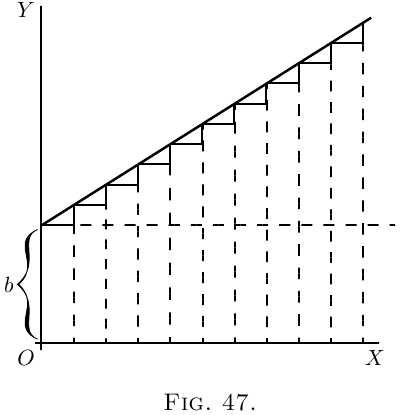
Go back to case (2) on here. Here we have the simplest of curves, a sloping line with the equation \[ y = ax+b. \]

We know that here $b$ represents the initial height of $y$ when $x= 0$, and that $a$, which is the same as $\dfrac{dy}{dx}$, is the “slope” of the line. The line has a constant slope. All along it the elementary triangles

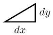
have the same proportion between height and base. Suppose we were to take the $dx$'s, and $dy$'s of finite magnitude, so that $10$ $dx$'s made up one inch, then there would be ten little triangles like

Now, suppose that we were ordered to reconstruct the “curve,” starting merely from the information that $\dfrac{dy}{dx} = a$. What could we do? Still taking the little $d$'s as of finite size, we could draw $10$ of them, all with the same slope, and then put them together, end to end, like this:

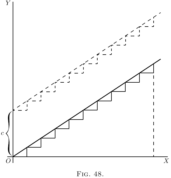
And, as the slope is the same for all, they would join to make, as in Figure 48, a sloping line sloping with the correct slope $\dfrac{dy}{dx} = a$. And whether we take the $dy$'s and $dx$'s as finite or infinitely small, as they are all alike, clearly $\dfrac{y}{x} = a$, if we reckon $y$ as the total of all the $dy$'s, and $x$ as the total of all the $dx$'s. But whereabouts are we to put this sloping line? Are we to start at the origin $O$, or higher up? As the only information we have is as to the slope, we are without any instructions as to the particular height above $O$; in fact the initial height is undetermined. The slope will be the same, whatever the initial height. 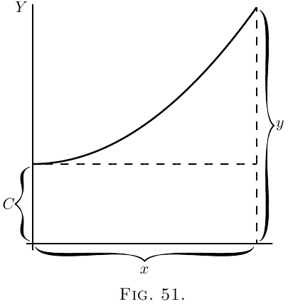Let us therefore make a shot at what may be wanted, and start the sloping line at a height $C$ above $O$. That is, we have the equation \[ y = ax + C. \]

It becomes evident now that in this case the added constant means the particular value that $y$ has when $x = 0$.

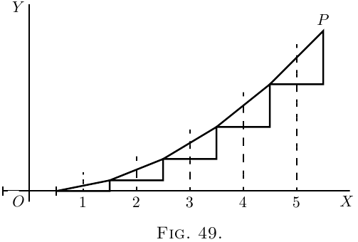
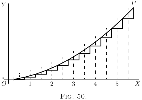
Now let us take a harder case, that of a line, the slope of which is not constant, but turns up more and more. Let us assume that the upward slope gets greater and greater in proportion as $x$ grows. In symbols this is: \[ \frac{dy}{dx} = ax. \] Or, to give a concrete case, take $a = \frac{1}{5}$, so that \[ \frac{dy}{dx} = \tfrac{1}{5} x. \]

Then we had best begin by calculating a few of the values of the slope at different values of $x$, and also draw little diagrams of them. When

Now try to put the pieces together, setting each so that the middle of its base is the proper distance to the right, and so that they fit together at the corners; thus (Figure 49). The result is, of course, not a smooth curve: but it is an approximation to one. If we had taken bits half as long, and twice as numerous, like Figure 50, we should have a better approximation. But for a perfect curve we ought to take each $dx$ and its corresponding $dy$ infinitesimally small, and infinitely numerous.

Then, how much ought the value of any $y$ to be? Clearly, at any point $P$ of the curve, the value of $y$ will be the sum of all the little $dy$'s from $0$ up to that level, that is to say, $\int dy = y$. And as each $dy$ is equal to $\frac{1}{5}x · dx$, it follows that the whole $y$ will be equal to the sum of all such bits as $\frac{1}{5}x · dx$, or, as we should write it, $\int \tfrac{1}{5}x · dx$.

Now if $x$ had been constant, $\int \tfrac{1}{5}x · dx$ would have been the same as $\frac{1}{5} x \int dx$, or $\frac{1}{5}x^2$. But $x$ began by being $0$, and increases to the particular value of $x$ at the point $P$, so that its average value from $0$ to that point is $\frac{1}{2}x$. Hence $\int \tfrac{1}{5} x\, dx = \tfrac{1}{10} x^2$; or $y=\frac{1}{10}x^2$.

But, as in the previous case, this requires the addition of an undetermined constant $C$, because we have not been told at what height above the origin the curve will begin, when $x = 0$. So we write, as the equation of the curve drawn in Figure 51, \[ y = \tfrac{1}{10}x^2 + C. \]

Exercises XVI